What is Time-Complexity?
So your program works, but it’s running too slow. Or maybe your nice little code is working out great, but it’s not running as quickly as that other lengthier one. Welcome to Big-O Time Complexity, where repetition is the enemy, and arrays reign supreme. I’m kidding…kind of. Big-O notation is a common means of describing the performance or complexity of an algorithm in Computer Science. Practically speaking, it is used as a barometer to test the efficiency of your function, and whether or not it can be improved upon. Time-Complexity will become an important aspect of your dev environment as your continue to progress through your studies. Eventually, you’ll be able to analyze your program and denote which programs fall within what time complexity (constant, linear, quadratic, exponential, logarithmic). In this guide, we’ll be breaking down the basics of Time-Complexity in order to gain a better understanding of how they look in your code and in real life.

O(1) — Constant Time:
Constant Time Complexity describes an algorithm that will always execute in the same time (or space) regardless of the size of the input data set. In JavaScript, this can be as simple as accessing a specific index within an array:

var array = [1, 2, 3, 4, 5];
array[0] // This is a constant time look-up
--------------------------------------------------------------------var removeLastElement = function(array) {
var numberOfElementsToRemove = 2;while (numberOfElementsToRemove > 0) {
array.pop();
}
}; //This will also have a constant time look-up since the function
//is only looking at a specific reference point within the array.

It doesn’t matter whether the array has 5 or 500 indices, looking up a specific location of the array would take the same amount of time, therefore the function has a constant time look-up.

In much the same way, if I had a deck of cards, and I asked you to remove the first any card at random, you could simply grab a card from the deck without having to search through the entire deck. That is a constant time look-up.

O(N)—Linear Time:
Linear Time Complexity describes an algorithm or program who’s complexity will grow in direct proportion to the size of the input data. As a rule of thumb, it is best to try and keep your functions running below or within this range of time-complexity, but obviously it won’t always be possible.

var numberRange = function(array) {
for (var i = 1; i < array.length; i++) {
console.log(array[i]);
}
}; //This will have a linear time look-up since the function is
//looking at a every index in the array once.

In this example, the look-up time is directly related to the size of our input because we will be going through each item within the array. In other words, the larger the input, the greater the amount of time it takes to perform the function. Of course, if the array only had 1 index (i.e. array.length === 1), then the function would have a constant time look-up.

Now, back to our deck of cards analogy. If I had a deck of cards and I wanted you to select a specific card (let’s say the 10❤s). You would have to look through every card until you found that card. Sure, there’s a possibility that it would be the first card in the deck, but that’s highly unlikely. Now think about if the deck of cards were filled with hundreds of other cards non-10❤ cards. Your search is directly related to how large the deck of cards is. That is an example of Linear Complexity.

O(log(n)) — Logarithmic Time:
Logarithmic Time Complexity refers to an algorithm that runs in proportionally to the logarithm of the input size. Now, if you haven’t worked with Binary Search Trees, this may be a little difficult to conceptualize, so I’ll try and demonstrate it clearly below.

//NOTE: This function is not an example of a Binary Search Tree
var partialRange = function(array) {
for (var i = 1; i < array.length; i = i * 2) {
console.log(array[i]);
}
}; //This will have a logarithmic time look-up since the function is
//looking at only searching through part of the array.

In the function above, we are logging numbers up until the array length is passed. However, we can see that our function will only be logging numbers at a certain interval. Since we will be repeating a constant time look-up on multiple parts of the array, our function will not have a constant time look up. It should also be noted that since our function does not pass through every index in the array, it will not have a linear time look-up.

Using our deck of cards analogy, let’s say our cards are ordered from increasing to decreasing order, with the deck split in half, one pile containing the clubs and spades, the other containing the hearts and diamond cards. Now, if I asked you to pull out the 10❤s, you could safely conclude that the card should be in the second pile, since that’s where the diamonds and hearts cards are. Furthermore, you know that the card should only be with the hearts, so you split the deck to only search through the heart cards. Since you’ll be searching for the 10❤s, you can safely assume that the bottom half of the deck is irrelevant (since they deck is already sorted). You can continue to split the remaining cards until you eventually find the 10❤s. You didn’t have to search through every card to find it, but it also wasn’t as easy as simply grabbing a random card. That is an example of Logarithmic Time Complexity.

O(N²) — Quadratic Time:
Quadratic Time Complexity represents an algorithm whose performance is directly proportional to the squared size of the input data set (think of Linear, but squared). Within our programs, this time complexity will occur whenever we nest over multiple iterations within the data sets.

var hasDuplicates = function(array) {
for (var i = 0; i < array.length; i++) {
var item = array[i];
if (array.slice(i + 1).indexOf(item) !== -1) {
return true;
}
}
return false;
}; //This will have a quadratic time look-up since the function is
//looking at a every index in the array twice.

This function is a great example of how easy it is to pass through an array twice without using two for loops. It’s clear in the first part that our function will be searching through the array at least once, but the difference-maker lies in the if statement. It is here where we are performing another look-up of the array with the native indexOf method. In doing so, we are passing over the same array twice with each search, producing a Quadratic Time Complexity.

Let’s revisit our deck of cards. Let’s say you picked the first card in the deck, and how to remove all the cards with that same number. You would have to search through the deck, removing the duplicates at every point. Once you were sure that all the duplicates were removed, you’d continue doing the same thing for second card, and third, and so on until you reached the end of the deck. This is an example of Quadratic Time Complexity.

O(2^N) — Exponential Time
Exponential Time complexity denotes an algorithm whose growth doubles with each additon to the input data set. If you know of other exponential growth patterns, this works in much the same way. The time complexity starts off very shallow, rising at an ever-increasing rate until the end.

var fibonacci = function(number) {
if (number <= 1) return number;
return Fibonacci(number - 2) + Fibonacci(number - 1);
}; //This will have an exponential time look-up since the function
//is looking at a every index an exponential number of times.

Fibonacci numbers are a great way to practice your understanding of recursion. Although there is a way to make the fibonacci function have a shorter time complexity, for this case we will be using the double recursive method to show how it has an Exponential Time Complexity. In a few words, the recursive instantiation will pass over every number from the number to zero. It will do this twice (once for each recursive call) until it reaches the base case if statement. Since the number of recursive calls is directly related to the input number, it is easy to see how this look-up time will quickly grow out of hand.

Before we begin, here are some things we already know about Javascript arrays:

• They are ordered.
• Use numbered indexing (zero-based indexes)
• Are dynamic.
• Data can be stored in non-contiguous locations in the array, so no guarantee of it being dense.
• Store multiple values in a single variable.

From a general view, these seem right as array properties, but to get more in-depth, Javascript arrays are constructed by the Array class, which is a global object, and arrays are referred to as high-level, list-like objects.

Yes, under the hood, Javascript Arrays are ‘objects’ and the quickest way to show this is by using typeof keyword:

typeof of an array in JS

You may have heard the statement “Almost everything in Javascript is an object or acts like one” or “If you understand objects, you’ve understood Javascript”

To show arrays are a special type of object, here is a code example:

assigning function to arr

In the above example, we have assigned a function to a property text and we can access it using the name ‘text’, which is what objects do - remember arrays are number indexed? But because JS arrays are objects under the hood, we can give arrays additional properties and access them by name.

Note: Just because that is possible does not mean it should be done:)

Quoting from MDN docs:

Setting or accessing via non-integers using bracket notation (or dot notation) will not set or retrieve an element from the array list itself, but will set or access a variable associated with that array’s object property collection. The array’s object properties and list of array elements are separate, and the array’s traversal and mutation operations cannot be applied to these named properties.

Another example:

Array.prototype.__proto__ vs Object.prototype

Array.prototype.__proto__ and Object.prototype are the same. This brings about the concept of prototype chaining. Quoting from the MDN docs:

Nearly all objects in JavaScript are instances of Object which sits on the top of a prototype chain.

The above is the reason Array instanceof Object returns true. Array is a constructor function, and Functions are objects in JS. You can read more about prototype-chaining here.

Time Complexity.

Javascript Array has methods to traverse and manipulate arrays. Some common ones are:

pop: Remove the item from the end of the array.

push: Add an item to the end of the array.

unshift: Add an item from the beginning of an array.

shift: Remove an item from the beginning of an array.

Adding/Removing Elements from the end of an array.

Array.push() and Array.pop() methods add/remove items from the end of the array. These have a Big O of constant time (O(1)) as they do not cause a shift in the index. They only add a new index for the new item at the end of the array.

Adding/Removing Elements from the start of an array.

Array.shift() and Array.unshift() methods add/remove items from the beginning of an array. These have a Big O of linear time (O(n)) as they cause an index shift for all other elements in the array i.e let’s say we have an array [1,2,3,4] , when we perform a shift method on it we now have [2,3,4] The index of 2 is now 0 when it was originally 1, the index of 3 is now 1 when it was originally 2 and so on. This shift is what causes the complexity of these methods to be linear.

This information is important especially as you write performant algorithms.

Code example:

shift vs pop performance

The above code makes use of NodeJS Performance Timing API. You can try it and see the time difference.

Traversing through an array.

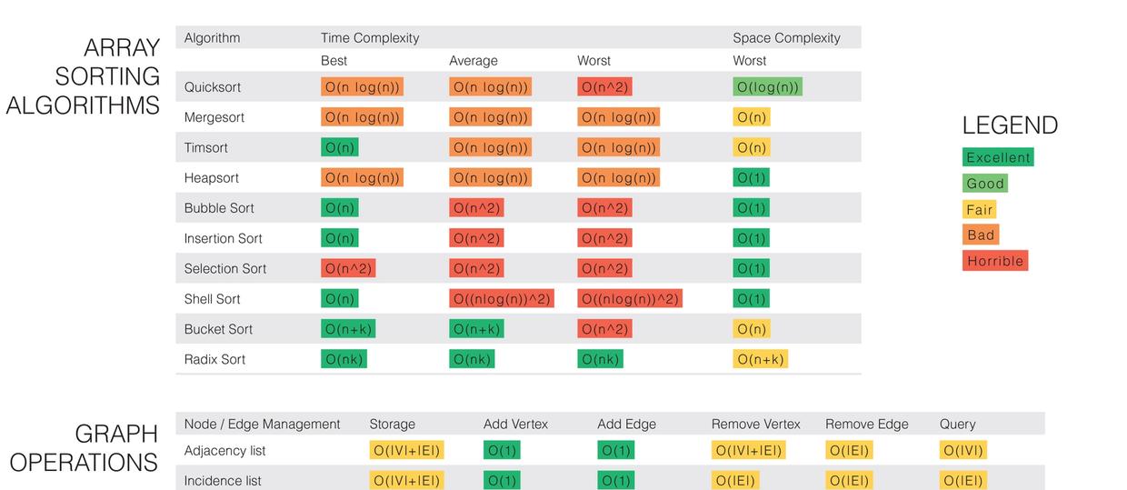
Array.reverse(), Array.reduce(), Array.forEach(), Array.filter(), Array.map(), Array.find() all have linear complexity.

Thinking through the time and space complexities of in built functions is very helpful when writing algorithms/solutions. Sometimes less code is actually slower code.

If you’ve ever looked into getting a job as a developer you’ve probably come across this Google interview at some point and wondered ‘what the heck are they talking about?’. In this article, we’re going to explore what they mean throwing around terms such as 'quadratic’ and 'n log n’.

In some of these examples I’m going to be referring to these two arrays, one with 5 items and another with 50. I’m also going to be using JavaScript’s handy performance API to measure the difference in execution time.

const smArr = [5, 3, 2, 35, 2]; const bigArr = [5, 3, 2, 35, 2, 5, 3, 2, 35, 2, 5, 3, 2, 35, 2, 5, 3, 2, 35, 2, 5, 3, 2, 35, 2, 5, 3, 2, 35, 2, 5, 3, 2, 35, 2, 5, 3, 2, 35, 2, 5, 3, 2, 35, 2, 5, 3, 2, 35, 2]; Copy

What is Big O Notation?

Big O notation is just a way of representing the general growth in the computational difficulty of a task as you increase the data set. While there are other notations, O notation is generally the most used because it focuses on the worst-case scenario, which is easier to quantify and think about. Worst-case meaning where the most operations are needed to complete the task; if you solve a rubik’s cube in one second you can’t say you’re the best if it only took one turn to complete.

As you learn more about algorithms you’ll see these expressions used a lot because writing your code while understanding this relationship can be the difference between an operation being nearly instantaneous or taking minutes and wasting, sometimes enormous amounts of, money on external processors like Firebase.

As you learn more about Big O notation, you’ll probably see many different, and better, variations of this graph. We want to keep our complexity as low and straight as possible, ideally avoiding anything above O(n).

O(1)

This is the ideal, no matter how many items there are, whether one or one million, the amount of time to complete will remain the same. Most operations that perform a single operation are O(1). Pushing to an array, getting an item at a particular index, adding a child element, etc, will all take the same amount of time regardless of the array length.

const a1 = performance.now(); smArr.push(27); const a2 = performance.now(); console.log(`Time: ${a2 - a1}`); // Less than 1 Millisecond const b1 = performance.now(); bigArr.push(27); const b2 = performance.now(); console.log(`Time: ${b2 - b1}`); // Less than 1 Millisecond Copy

O(n)

By default, all loops are an example of linear growth because there is a one-to-one relationship between the data size and time to completion. So an array with 1,000 times more items will take exactly 1,000 times longer.

const a1 = performance.now(); smArr.forEach(item => console.log(item)); const a2 = performance.now(); console.log(`Time: ${a2 - a1}`); // 3 Milliseconds const b1 = performance.now(); bigArr.forEach(item => console.log(item)); const b2 = performance.now(); console.log(`Time: ${b2 - b1}`); // 13 Milliseconds Copy

O(n^2)

Exponential growth is a trap we’ve all fall into at least once. Need to find a matching pair for each item in an array? Putting a loop inside a loop is great way of turning an array of 1,000 items into a million operation search that’ll freeze your browser. It’s always better to have to do 2,000 operations over two separate loops than a million with two nested loops.

const a1 = performance.now(); smArr.forEach(() => { arr2.forEach(item => console.log(item)); }); const a2 = performance.now(); console.log(`Time: ${a2 - a1}`); // 8 Milliseconds const b1 = performance.now(); bigArr.forEach(() => { arr2.forEach(item => console.log(item)); }); const b2 = performance.now(); console.log(`Time: ${b2 - b1}`); // 307 Milliseconds Copy

O(log n)

The best analogy I’ve heard to understand logarithmic growth is to imagine looking up a word like 'notation’ in a dictionary. You can’t search one entry after the other, instead you find the 'N’ section, then maybe the 'OPQ’ page, then search down the list alphabetically until you find a match.

With this 'divide-and-conquer’ approach, the amount of time to find something will still change depending on the size of the dictionary but at nowhere near the rate of O(n). Because it searches in progressively more specific sections without looking at most of the data, a search through a thousand items may take less than 10 operations while a million may take less than 20, getting you the most bang for your buck.

In this example, we can do a simple quicksort.

const sort = arr => { if (arr.length < 2) return arr; let pivot = arr[0]; let left = []; let right = []; for (let i = 1, total = arr.length; i < total; i++) { if (arr[i] < pivot) left.push(arr[i]); else right.push(arr[i]); }; return [ ...sort(left), pivot, ...sort(right) ]; }; Copysort(smArr); // 0 Milliseconds sort(bigArr); // 1 Millisecond Copy

O(n!)

Finally, one of the worst possibilities, factorial growth. The textbook example of this is the travelling salesman problem. If you have a bunch of cities of varying distance, how do you find the shortest possible route that goes between all of them and returns to the starting point? The brute force method would be to check the distance between every possible configuration between each city, which would be a factorial and quickly get out of hand.

Since that problem gets very complicated very quickly, we’ll demonstrate this complexity with a short recursive function. This function will multiply a number by its own function taking in itself minus one. Every digit in our factorial will run its own function until it reaches 0, with each recursive layer adding its product to our original number. So 3 is multiplied by 2 that runs the function to be multiplied by 1 that runs it again to be stopped at 0, returning 6. Recursion gets confusing like this pretty easily.

A factorial is just the product of every number up to that number. So 6! is 1x2x3x4x5x6 = 720.

const factorial = n => { let num = n; if (n === 0) return 1 for (let i = 0; i < n; i++) { num = n * factorial(n - 1); }; return num; }; Copyfactorial(1); // 2 Milliseconds factorial(5); // 3 Milliseconds factorial(10); // 85 Milliseconds factorial(12); // 11,942 Milliseconds Copy

I intended on showing factorial(15) instead but anything above 12 was too much and crashed the page, thus proving exactly why this needs to be avoided.

What is algorithm analysis anyway, and why do we need it??

Before diving into algorithm complexity analysis, let’s first get a brief idea of what algorithm analysis is. Algorithm analysis deals with comparing algorithms based upon the number of computing resources that each algorithm uses.

What we want to achieve by this practice is being able to make an informed decision about which algorithm is a winner in terms of making efficient use of resources(time or memory, depending upon use case). Does this make sense?

Let’s take an example. Suppose we have a function product() which multiplies all the elements of an array, except the element at the current index, and returns the new array. If I am passing [1,2,3,4,5] as an input, I should get [120, 60, 40, 30, 24] as the result.

The above function makes use of two nested for loops to calculate the desired result. In the first pass, it takes the element at the current position. In the second pass, it multiplies that element with each element in the array — except when the element of the first loop matches the current element of the second loop. In that case, it simply multiplies it by 1 to keep the product unmodified.

Are you able to follow? Great!

It’s a simple approach which works well, but can we make it slightly better? Can we modify it in such a way that we don’t have to make two uses of nested loops? Maybe storing the result at each pass and making use of that?

Let’s consider the following method. In this modified version, the principle applied is that for each element, calculate the product of the values on the right, calculate the products of values on the left, and simply multiply those two values. Pretty sweet, isn’t it?

Here, rather than making use of nested loops to calculate values at each run, we use two non-nested loops, which reduces the overall complexity by a factor of O(n) (we shall come to that later).

We can safely infer that the latter algorithm performs better than the former. So far, so good? Perfect!

At this point, we can also take a quick look at the different types of algorithm analysis which exist out there. We do not need to go into the minute level details, but just need to have a basic understanding of the technical jargon.

Depending upon when an algorithm is analyzed, that is, before implementation or after implementation, algorithm analysis can be divided into two stages:

• Apriori Analysis − As the name suggests, in apriori(prior), we do analysis (space and time) of an algorithm prior to running it on a specific system. So fundamentally, this is a theoretical analysis of an algorithm. The efficiency of an algorithm is measured under the assumption that all other factors, for example, processor speed, are constant and have no effect on the implementation.
• Apostiari Analysis − Apostiari analysis of an algorithm is performed only after running it on a physical system. The selected algorithm is implemented using a programming language which is executed on a target computer machine. It directly depends on system configurations and changes from system to system.

In the industry, we rarely perform Apostiari analysis, as software is generally made for anonymous users who might run it on different systems.
Since time and space complexity can vary from system to system, Apriori Analysis is the most practical method for finding algorithm complexities. This is because we only look at the asymptotic variations (we will come to that later) of the algorithm, which gives the complexity based on the input size rather than system configurations.

Now that we have a basic understanding of what algorithm analysis is, we can move forward to our main topic: algorithm complexity. We will be focusing on Apriori Analysis, keeping in mind the scope of this post, so let’s get started.

Deep dive into complexity with asymptotic analysis

Algorithm complexity analysis is a tool that allows us to explain how an algorithm behaves as the input grows larger.

So, if you want to run an algorithm with a data set of size n, for example, we can define complexity as a numerical function f(n) — time versus the input size n.

Time vs Input

Now you must be wondering, isn’t it possible for an algorithm to take different amounts of time on the same inputs, depending on factors like processor speed, instruction set, disk speed, and brand of the compiler? If yes, then pat yourself on the back, cause you are absolutely right!?

This is where Asymptotic Analysis comes into this picture. Here, the concept is to evaluate the performance of an algorithm in terms of input size (without measuring the actual time it takes to run). So basically, we calculate how the time (or space) taken by an algorithm increases as we make the input size infinitely large.

Complexity analysis is performed on two parameters:

1. Time: Time complexity gives an indication as to how long an algorithm takes to complete with respect to the input size. The resource which we are concerned about in this case is CPU (and wall-clock time).
2. Space: Space complexity is similar, but is an indication as to how much memory is “required” to execute the algorithm with respect to the input size. Here, we dealing with system RAM as a resource.

Are you still with me? Good! Now, there are different notations which we use for analyzing complexity through asymptotic analysis. We will go through all of them one by one and understand the fundamentals behind each.

The Big oh (Big O)
The very first and most popular notation used for complexity analysis is BigO notation. The reason for this is that it gives the worst case analysis of an algorithm. The nerd universe is mostly concerned about how badly an algorithm can behave, and how it can be made to perform better. BigO provides us exactly that.

Let’s get into the mathematical side of it to understand things at their core.

BigO (tightest upper bound of a function)

Let’s consider an algorithm which can be described by a function f(n). So, to define the BigO of f(n), we need to find a function, let’s say, g(n), which bounds it. Meaning, after a certain value, n0, the value of g(n) would always exceed f(n).

We can write it as,
f(n) ≤ C g(n)
where n≥n0; C> 0; n0≥1

If above conditions are fulfilled, we can say that g(n) is the BigO of f(n), or
f(n) = O (g(n))

Can we apply the same to analyze an algorithm? This basically means that in worst case scenario of running an algorithm, the value should not pass beyond a certain point, which is g(n) in this case. Hence, g(n) is the BigO of f(n).

Let’s go through some commonly used bigO notations and their complexity and understand them a little better.

• O(1): Describes an algorithm that will always execute in the same time (or space) regardless of the size of the input data set.

function firstItem(arr){ return arr[0];}

The above function firstItem(), will always take the same time to execute, as it returns the first item from an array, irrespective of its size. The running time of this function is independent of input size, and so it has a constant complexity of O(1).

Relating it to the above explanation, even in the worst case scenario of this algorithm (assuming input to be extremely large), the running time would remain constant and not go beyond a certain value. So, its BigO complexity is constant, that is O(1).

• O(N): Describes an algorithm whose performance will grow linearly and in direct proportion to the size of the input data set. Take a look at the example below. We have a function called matchValue() which returns true whenever a matching case is found in the array. Here, since we have to iterate over the whole of the array, the running time is directly proportional to the size of the array.

function matchValue(arr, k){ for(var i = 0; i < arr.length; i++){ if(arr[i]==k){ return true; } else{ return false; } } }

This also demonstrates how Big O favors the worst-case performance scenario. A matching case could be found during any iteration of the for loop and the function would return early. But Big O notation will always assume the upper limit (worst-case) where the algorithm will perform the maximum number of iterations.

• O(N²): This represents an algorithm whose performance is directly proportional to the square of the size of the input data set. This is common with algorithms that involve nested iterations over the data set. Deeper nested iterations will result in O(N³), O(N⁴), etc.

function containsDuplicates(arr){ for (var outer = 0; outer < arr.length; outer++){ for (var inner = 0; inner < arr.length; inner++){ if (outer == inner) continue; if (arr[outer] == arr[inner]) return true; } } return false;}

• O(2^N): Denotes an algorithm whose growth doubles with each addition to the input data set. The growth curve of an O(2^N) function is exponential — starting off very shallow, then rising meteorically. An example of an O(2^N) function is the recursive calculation of Fibonacci numbers:

function recursiveFibonacci(number){ if (number <= 1) return number; return recursiveFibonacci(number - 2) + recursiveFibonacci(number - 1);}

Are you getting the hang of this? Perfect. If not, feel free to fire up your queries in the comments below. :)

Moving on, now that we have a better understanding of the BigO notation, let us get to the next type of asymptotic analysis which is, the Big Omega(Ω).

The Big Omega (Ω)?
The Big Omega(Ω) provides us with the best case scenario of running an algorithm. Meaning, it would give us the minimum amount of resources (time or space) an algorithm would take to run.

Let’s dive into the mathematics of it to analyze it graphically.

BigΩ (tightest lower bound of a function)

We have an algorithm which can be described by a function f(n). So, to define the BigΩ of f(n), we need to find a function, let’s say, g(n), which is tightest to the lower bound of f(n). Meaning, after a certain value, n0, the value of f(n) would always exceed g(n).

We can write it as,
f(n)≥ C g(n)
where n≥n0; C> 0; n0≥1

If above conditions are fulfilled, we can say that g(n) is the BigΩ of f(n), or
f(n) = Ω (g(n))

Can we infer that Ω(…) is complementary to O(…)? Moving on to the last section of this post…

The Big Theta (θ)?
The Big Theta(θ) is a sort of a combination of both BigO and BigΩ. It gives us the average case scenario of running an algorithm. Meaning, it would give us the mean of the best and worst case. Let’s analyse it mathematically.

Bigθ (tightest lower and upper bound of a function)

Considering an algorithm which can be described by a function f(n). The Bigθ of f(n) would be a function, let’s say, g(n), which bounds it the tightest by both lower and upper bound, such that,
C₁g(n) ≤ f(n)≤ C₂ g(n)
where C₁, C₂ >0, n≥ n0,
n0 ≥ 1

Meaning, after a certain value, n0, the value of C₁g(n) would always be less than f(n), and value of C₂ g(n) would always exceed f(n).

Now that we have a better understanding of the different types of asymptotic complexities, let’s have an example to get a clearer idea of how all this works practically.

Consider an array, of size, say, n, and we want to do a linear search to find an element x in it. Suppose the array looks something like this in the memory.

Linear Search

Going by the concept of linear search, if x=9, then that would be the best case scenario for the following case (as we don’t have to iterate over the whole array). And from what we have just learned, the complexity for this can be written as Ω(1). Makes sense?

Similarly, if x were equal to 14, that would be the worst case scenario, and the complexity would have been O(n).

What would be the average case complexity for this?
θ(n/2) => 1/2 θ(n) => θ(n) (As we ignore constants while calculating asymptotic complexities).

ime complexity simply refers to the amount of time it takes an algorithm, or set of code, to run.

Time complexity is most often measured in Big O notation. If you’re unfamiliar with Big O, here’s a great article that breaks it down in simple terms. For my includesDouble function, n, which is the size of the input, would be 3 — if we were to use either of our earlier arrays ([3, 4, 6] OR [4, 5, 7]). So we begin with O(n) = 3.

When considering time complexity, best practice is to calculate the worst case scenario. Looking at our two arrays, that would be [4, 5, 7], because we know that this array does not include a double, so both loops (our while loop and .includes()) will run completely through the entire array because there is no true case that will break them out of the loops. Okay, so if [4, 5, 7] runs through the while loop we have a linear run time of O(n) = 3, because our while loop runs once for each element in our array (once for 4, twice for 5, and a third time for 7). However, for each iteration of our while loop we have a nested loop that also runs — .includes().

Beware of nested loops — this is where your time complexity, or Big O notation, begins to grow exponentially.

Let me explain…

If our array includes the numbers 4, 5, and 7, on our first iteration through (where array[i] = 4), our .includes() method is going to run through each item in our array to see if the array includes 8 (array[i] * 2). It will then do the same thing for all of the other numbers in our array (5, then 7).

To make things more explicit, our JavaScript engine would run through the following steps:

1. For the number 4, does 4 equal 8?
2. For the number 4, does 5 equal 8?
3. For the number 4, does 7 equal 8?
4. For the number 5, does 4 equal 10?
5. For the number 5, does 5 equal 10?
6. For the number 5, does 7 equal 10?
7. For the number 7, does 4 equal 14?
8. For the number 7, does 5 equal 14?
9. For the number 7, does 7 equal 14?

Because we have a nested loop, our Big O notation goes from O(n) = 3 to O(n²) = 3². A Big O of 3 vs. a Big O of 9 isn’t that great a difference, but remember that with time complexity, we want to consider the worst case scenario — what if our array was a thousand numbers long? All of a sudden, O(n) = 1000, turns to O(n²) = 1,000,000 with a nested loop! Now that’s a big difference! Imagine if our array contained a million numbers!!!

So, is there a way to solve this problem with an algorithm that doesn’t use a nested loop?

I’m so glad you asked, because the answer is yes.

Enter the hash table…

A hash table is simply a data structure that is associative — it maps keys to values.

If you’ve been coding for at least a little while, you’ll have seen this type of data structure before — (hash tables are also called objects in JavaScript and hashes in Ruby).

‘That’s really great,’ you’re probably thinking — ‘but how does a hash table about cats solve the algorithm problem above?’

Let me share with you the solution first, and then we’ll go through it step by step.

Again, we’ll use our previous array ([4, 5, 7]) to walk through this function.

On the first line inside the function, notice that I’m declaring a new variable, doubles, and setting it equal to an empty hash table ({}). We’re going to build out this hash table using the elements from our array as we go.

Just as before, we’ll start with a while loop (O(n) = 3). Inside the while loop, I’m going to use the numbers in my array to make keys for my new hash table (doubles[array[i]] = ‘cats are so cool’). We know that with this array, our while loop will return without returning true, so after our while loop finishes, we’ll have a hash table that looks like this:

Cats ARE really, really cool.

Notice that, even though they’re full of wisdom, the values that I’ve set my keys to don’t really matter. The keys are the key.

Now let’s look at the second line in our while loop — here we have another conditional — only this time we’re not using .includes(). Instead, we’re checking the keys in our hash table against our current number to see if there is a key that is already double, or half of, our current number. If that key already exists, then we know that we’ve found a double!

To break it down more explicitly…

1. Our first run through the while loop (with array[i] = 4) produces doubles = {4: ‘cats are so cool’}. It runs through the conditional without returning anything because doubles has only one key, 4, and does not include a key of 8 or 2.
2. The second run through the while loop (with array[i] = 5) adds a new key to doubles — {4: ‘cats are so cool’, 5: ‘cats are so cool’}. Again it passes through the conditional without matching a key.
3. Finally, our last run through produces doubles = {4: ‘cats are so cool’, 5: ‘cats are so cool’, 7: ‘cats are so cool’} and exits the conditional and the while loop without matching a key.
4. Because there was no positive case to break us out of the while loop, our function returns false!

Notice anything?

We wrote a function that does what it needs to do without using a nested loop!

The Big O notation for this version of our includesDouble function is just O(n) = 3. If we had an array of a million numbers, Big O would be O(n) = 1,000,000. Compare that with O(n²) = 1,000,000,000,000 (one trillion) and we’ve shaved off a huge chunk of our function’s run time!

Ahhh… isn’t life good?

As great as our new function is, it does pose some trade-offs — first of all, our second function is a little harder to understand than our first. If you’re concerned about readability (maybe you’ve got a bunch of newbie programmers on your staff, like me) and you know that n is never going to be astronomically long, you may prefer to stick with the first option. Also, notice that in the second function we also create a brand new variable (doubles = {}). This means that your computer now has to create and set aside a specific place in memory to store that new piece of data. If you’re worried about memory space, and you know that n will always be a reasonable length, again you may choose to go with option #1.